Demystifying the Analemma
Contents
Here’s complete Analemma calculator if you want to see it in action before delving into the specifics.
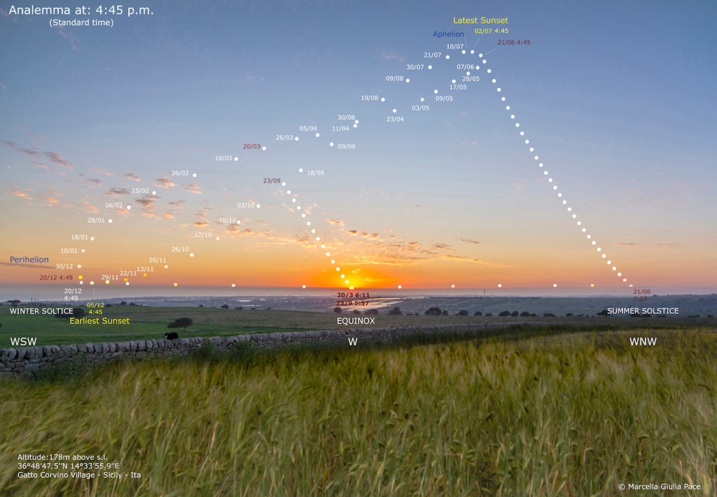
If you were to take a picture of the Sun every day, at the same time, for an entire year, it would form a figure eight shaped loop. It’s a surprisingly tricky astronomical phenomena to photograph, because you need to take the more than three hundreds pictures at the same location with the same setup to get optimal results. There’s also the challenge of dealing with an unpredictable weather.
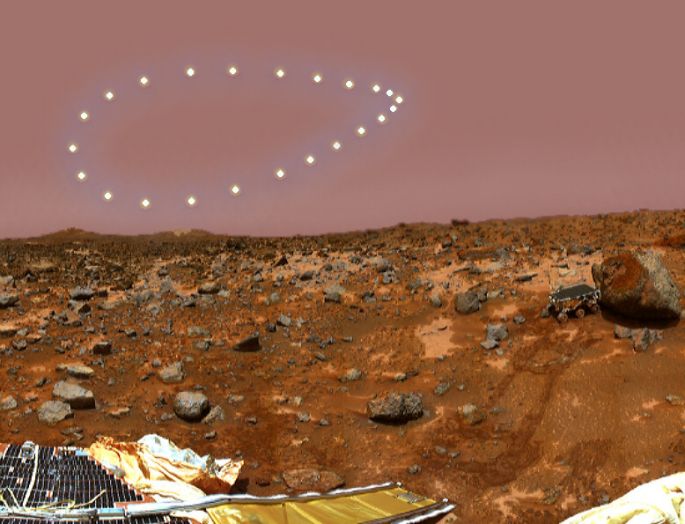
Analemmas aren’t unique to planet Earth. Planets have different shapes according to their different inclinations and orbits.
Thankfully, we don’t need to spend a year to know how Analemmas look and work. Today is the march equinox, the day where the sun passes directly over the equator, so I think it’s the perfect opportunity to talk about analemmas.
Why does it look like that? Why a figure eight? Why is Mars’ analemma so different? These were some of the questions I had that made me wonder about that weird looking shape. I didn’t want a formula or equation for calculating it. I wanted to know why. I wanted to generalize the analemma for every possible orbit.
It seems daunting, I know, but bear with me. You might learn one or two things about celestial mechanics and geometry.
First of all, why does the sun need to be photographed every twenty four hours? Why not every twelve hours? Every hour? Every minute? Well, it’s a simple trick to cancel the Earth’s own rotation. The Earth is rotating, so the sun changes its position in the sky regardless of the Earth’s orbital parameters. In fact, if the Earth were tidally locked to the sun, you would be able to film the analemma over a year.
However, the Earth spins roughly every twenty four hours, so we need to wait for the sun to return to the position it had before taking another picture.
The Mean Sun
Let’s consider the most simple analemma: A single point in the sky. In this hypothetical case the sun would be at the same place in the sky. During local noon, at the equator, the sun would be directly overhead, for example. Throughout a year, at the same time, the sun would remain at the same place. A boring analemma indeed.
This analemma is possible if:
- The orbit of the planet were perfectly circular
- The planet had no axial tilt
That means the sun would always be directly above the equator. This is the “mean” or average sun. A perfect sun that moves at a constant rate. Always in the same position every day, always in time. This is perfect for timekeeping, unfortunately, the real sun is not so perfect. Earth’s orbit is elliptical, and the planet itself is tilted.
The analemma is a measure of how much the true sun deviates from the mean sun. That figure eight shape is a sort of “signature” that encodes the planet’s orbital parameters and axial tilt.
Calculating the analemma is useful for knowing the difference between the ideal or mean solar clock and the real, or apparent one.
The analemma has two components:
- The vertical component, caused by the planet’s axial tilt
- The horizontal component, caused by the planet’s orbital eccentricity and axial tilt
Declination
As the Earth revolves around the sun, it keeps a constant tilt of approximately 23.4° degrees with respect to the plane of its orbit. During the summer in the northern hemisphere, for example, the top part of the planet receives the most sunlight, and days tend to be longer, because the sun now reaches a higher point in the sky. Near the poles, you can experience continuous sunlight for more than a day!
The opposite happens half an orbit later. The southern hemisphere starts to receive more sunlight, and winter begins in the north. Days are now shorter, and the sun appear to be lower in the sky.
The more tilted a planet is, the vertical component of the analemma, its declination, increases. Not only that, but also the way it increases changes.
This is an approximation of the solar declination:
\[\delta = \epsilon \sin(\theta)\]
- \(\delta\): Apparent solar declination
- \(\epsilon\): Axial tilt
- \(\theta\): Angular position of the planet along its orbit
However, this is only accurate for a small axial tilt. As the axial tilt approaches 90°, it gets less and less accurate. A more correct equation would be:
\[\delta = \sin^{-1} (\sin(\epsilon) \sin(\theta))\]
Both functions are compared below:
Notice how at small angles, the declination approximates a sine wave. As we increase the axial tilt, it starts to behave like a triangle wave.
The analemma spans 46.8° on the vertical axis, oscillating as the planet changes its apparent declination. The vertical components reaches a maximum or minimum during the solstices, and it’s exactly zero at the equinoxes. With the mystery of the vertical movement of the sun solved, it’s time to explain the horizontal movement of the sun.
The Equation of Time
The equation of time is a function that tells us how much our definition of a day (mean solar time), deviates from the true solar time. It is the function that dictates the horizontal movement of the analemma.
It has two components, caused by two variables:
- Eccentricity (\(e\)): Since the Earth’s movement along its orbit is not constant,
sometimes it will me moving faster or slower than the mean solar time. If the Earth had an eccentricity of zero, this component of the equation of time would also be zero.
- Obliquity (\(\epsilon\)): The obliquity is the parameter that gives the
analemma its figure eight shape. As the solar declination changes, a small horizontal component is added to the equation of time.
To explain the effect of eccentricity, we’ll first define an orbit.
Defining an orbit
This is a very simple formula for plotting an orbit with one of its foci at the origin, with perihelion starting at \(\theta = 0\)
\[f(\theta) = \begin{cases}x = a (\cos \theta - e) \\ y = a \sqrt{1 - e^2} \cdot \sin \theta \end{cases}\]
In this case, \(a\) is the semi-major axis and \(e\) the orbital eccentricity.
The Three Anomalies
Now that we have the shape of the orbit, it’s time to place the planet on it. The questions is where, and when?
Two angles can help us determine the effect of the eccentricity of the equation of time
- Mean anomaly: It’s an angular quantity that increases linearly with time. This is the “mean solar time” we’re measuring against.
- True anomaly: It’s the angle that represents the true position of a planet. If an orbit were perfectly circular, it would be equal to the mean anomaly (Time difference of zero).
The true anomaly does not increase linearly with time, due to the eccentricity of the orbit which makes our hypothetical planet move faster near perihelion and slower near aphelion. We use mean solar time because it’s linear and easy to calculate, however it deviates from the apparent solar time. If Earth’s eccentricity were larger it would be a larger difference.
Finally, the eccentric anomaly will allow us to plot the planet’s position using the equation shown above.
The mean anomaly is the easiest to calculate, it completes a full revolution (\(2\pi\) radians) every orbital period.
\[M = \frac{2 \pi t}{T}\]
The mean anomaly can also be calculated from the eccentric anomaly:
\[M = E - e \sin(E)\]
Where \(e\) is the orbital eccentricity. Note that if \(e\) were zero, \(E\) would be equal to \(M\).
To get the true anomaly from the eccentric anomaly:
\[\nu = \tan^{-1} \left ( \frac{\sqrt{1 - e^2} \sin(E)}{\cos(E) - e} \right )\]
Again, if \(e\) were zero, \(\nu\) would be equal to \(E\).
The problem lies in solving \(E\) in terms on \(M\), which can only be done numerically using Newton’s method:
\[E_1 = M\]
\[E_{n + 1} = E_n - \frac{E_n - e \sin(E_n) - M}{1 - e \cos(E_n)}\]
It’s necessary to calculate several iterations of \(E\) to get an accurate value.
Once we have the eccentric anomaly, we can calculate the true anomaly of our orbiting body. The eccentric anomaly can be plugged in this equation to obtain the position of the body.
With the position \((x, y)\) calculated, the true anomaly can also be calculated with:
\[\nu = \text{atan2}(y, x)\]
The Vernal Equinox
Imagine the Earth had a very eccentric orbit. Ignoring the effects on the climate and the fact that the seasons would now be primarily determined by the extreme variations in distance, consider what would happen during spring in the northern hemisphere exactly at perihelion. Near perihelion, Earth would move a lot faster, making spring and winter very short, and summer and autumn very long. This means the declination is also affected by the orbital eccentricity. Things complicate when we change the tilt of the Earth so that spring begins at a point other than perihelion or aphelion.
The vernal equinox is used as a reference that marks the beginning of spring in the northern hemisphere.
Now, our updated formula for the declination looks like:
\[\delta = \sin^{-1} (\sin(\epsilon) \sin(\nu - V))\]
- \(\delta\): solar declination angle
- \(\epsilon\): Axial tilt
- \(\nu\): True anomaly
- \(V\): Vernal equinox
For this equation, a vernal equinox of 0° would mean spring in the northern hemisphere begins exactly at perihelion.
So how would the declination over time look like when we take into account the effects of orbital eccentricity? The graph below shows it.
Note that with an orbital eccentricity of zero, changing the vernal equinox only translates the declination function in the horizontal axis. However, once the eccentricity is increased significantly, its effect on the solar declination becomes noticeable.
By tuning these three values (the eccentricity, axial tilt and vernal equinox), you can obtain extremely long summers and short winters, for example.
Putting it all together
These are the following parameters we’ve reviewed so far that affect the shape of the analemma:
- The planet’s obliquity
- The eccentricity of its orbit
- The angle between perihelion and the vernal equinox
There are several equations that can help us calculate the equation or time and declination at any given point. However, my goal with this calculator is to try to avoid magic numbers. Instead, seeing an orbit and a planet in motion would allow us to see exactly how each of these parameters affects the shape of the analemma.
The analemma as a function of time can be defined as:
\[A(t) \begin{cases} x = \text{EoT}(t) \\ y = \text{Dec}(t) \end{cases}\]
where \(\text{EoT}\) is the equation of time and \(\text{Dec}\) the solar declination, both in degrees. The equation of time is also usually measured in minutes, that correspond to the actual time difference between the mean and true sun. However, they can be converted to an angular quantity.
Declination
\[\text{Dec}(t) = \sin^{-1} (\sin(\epsilon) \sin(\nu(t) - V))\]
\[M(t) = \frac{2 \pi t}{T}\]
\[\nu(t) = \tan^{-1} \left ( \frac{\sqrt{1 - e^2} \sin(E(t))}{\cos(E(t)) - e} \right )\]
And finally, to get \(E(t)\) we can resort to numerical methods.
\[E_1(t) = M(t)\]
\[E_{n + 1} = E_n(t) - \frac{E_n(t) - e \sin(E_n(t)) - M(t)}{1 - e \cos(E_n(t))}\]
\[E(t) = E_k(t)\]
In this case, \(k\) can be an arbitrary number of iterations (the more the better).
Equation of Time
An initial approximation of the equation of time can be:
\[\text{EoT}(t) = M(t) - \nu(t)\]
However this doesn’t take into account the effect of obliquity. When projecting the true sun on the equatorial plane, there’s an angular difference between the projection and the mean sun.
\[\text{EoT}(t) = M(t) - V - \text{atan2}\left (\sin(\nu(t) - V) \cos(\epsilon), \cos(\nu(t) - V) \right )\]
Note that if the obliquity \(\epsilon = 0\):
\[\text{EoT}(t) = M(t) - V - \text{atan2}\left (\sin(\nu(t) - V), \cos(\nu(t) - V) \right )\]
\[\text{EoT}(t) = M(t) - V - (\nu(t) - V)\]
\[\text{EoT}(t) = M(t) - \nu(t)\]
These formulas may give us a nice analemma, but it’s difficult to visualize them. The equations are only one side of the story. Wouldn’t it be nice to see the equations in a different, more intuitive way?
Defining the Celestial Sphere
The celestial sphere is a useful model for understanding and visualizing different astronomical phenomena. The seasons, the plane of the ecliptic, the subsolar point, and even the positions of other stars!
For this SVG model, the XY plane represents the equatorial plane that the mean sun circles over an orbital period. In the center we have the planet itself, happily rotating on its own axis.
Changing the obliquity slider will change the inclination of the ecliptic. The apparent sun is always on this plane, and only intersects the equatorial plane during the equinoxes. It reaches its highest or lowest point during the solstices.
The analemma is traced on both the celestial sphere and on the planet’s surface. On the surface, it represents the location where the sun is directly overhead.